Excel pie chart group small values
Written by co-founder Kasper Langmann Microsoft Office Specialist. The right panel shows all the data a little too compressed to make out a slope in the small.

Rule 6 Arrange Your Pie Slices From Largest To Smallest Addtwo
Click Save to save the chart as a chart template crtx Download 25 Excel Chart Templates.
. To find the chart and graph options select Insert. Compacting the task bars will make your Gantt graph look even better. Click on any remaining labels that are on the small pie to select them and press the delete button on your keyboard to get rid of them.
So visualizing data using charts that display hierarchical insights can help you persuade your target audience or readers. Change all positive signs to negative and reverse the sign of all values. Position This option lets you specify the number of positions that you want to move to the stacked chart.
Compare a normal pie chart before. Because its so useful. Value This option lets you specify the maximum values that will be displayed in the pie chart.
A bubble chart in excel might be difficult for a user. In fact I will go ahead and say that pie charts are actually the most widely used charts in business contexts. Pie-of-pie and bar-of-pie charts make it easier to see small slices of a pie chart.
Next find the Pie charts and pick whichever chart you like the best. To create a Pie chart in Excel you need to have your data structured as shown below. Change Sign of Values.
Or click the Chart Filters button on the right of the graph and then click the Select Data link at the bottom. Creating Pie of Pie Chart in Excel. This will create an Excel pivot table group by week.
They primarily show how different values add up to a whole. Remove excess white space between the bars. When you return to Word click Refresh Data to update your chart to reflect any changes made to the data in Excel.
How to Make Pie Chart in Excel with Subcategories 2 Quick Methods Conclusion. Excel 2013 and above versions are required to use this chart template. To create a chart template in Excel do the following steps.
This article covers all the necessary things regarding Excel Pie Chart. See how Excel identifies each one in the top navigation bar as depicted below. Click on the chart youve just created to activate the Chart Tools tabs on the Excel ribbon go to the Design tab Chart Design in Excel 365 and click the Select Data button.
With this Excel utility you can easily fix trailing negative signs. A bubble chart is a variation of a scatter chart in which the data points are replaced with bubbles and an additional dimension of the data is represented in the size of the bubbles. A new chart will appear.
Advantages of Bubble chart in Excel. Click any of the orange bars to get them all selected right click and select Format Data Series. Last now we dont know which piece of the pie represents which stock.
Create a chart and customize it 2. Now look at the Format tab. You can find the add-in under the Insert Tab Select the data range then click on the people graph icon.
Attractive Bubbles of different sizes will catch the readers attention easily. Jon Peltier can stand on his roof and shout in to a megaphone Use Bar Charts Not Pies but the fact remains that most of us use pie charts sometime or other. Hope after reading this article you will not face any difficulties with the pie chart.
Percentage value This option lets you specify the minimum percentage for portions to be moved to the stacked chart. Just like a scatter chart a bubble chart does not use a category axis both horizontal and vertical axes are value axes. Pareto chart also called a Pareto diagram is a graph based on the Pareto principle.
Values less than this will be moved to the stacked bar. Click on the drop-down menu of the pie chart from the list of the charts. In addition to the x values and y values that are plotted in a scatter chart a bubble.
This will Excel group by week every 7 days starting on a Monday. Right click on the lines leading from the big pie to the now invisible small pie and select no line. This is where a Sunburst Chart in Excel comes in.
To add this information click your pie chart then at the top of the page click Design. You can also go into Excel by double-clicking your chart. The pie chart is one of the most commonly used charts in Excel.
Today I want to teach you a simple pie chart hack that can improve readability of the chart. Under Fill click Solid Fill and choose the background color from the paint bucket icon in the Font group. In Excel your options for charts and graphs include column or bar graphs line graphs pie graphs scatter plots and more.
The so-called Comparison Group. And here is the result of our efforts - a simple but nice. In the example below a pie-of-pie chart adds a secondary pie to show the three smallest slices.
In the VALUES area put in the Sales field. Change Chart Type allows you to switch from a pie chart to a line graph and so on using the same set of data. These chart types separate the smaller slices from the main pie chart and display them in a secondary pieor stacked bar chart.
A pie chart sometimes called a circle chart is a useful tool for displaying basic statistical data in the shape of a circle each section resembles a slice of pieUnlike in bar charts or line graphs you can only display a single data series in a pie chart and you cant use zero or negative values when creating oneA negative value will display as its positive equivalent and a. The description of the pie slices should be in the left column and the data for each slice should be in the right column. This will get the total of the Sales for each 7-day date range you have defined.
The bubble chart in excel is visually better than the table format. The article provides free Excel chart resources. Its nonsensical to talk about trends with categorical labels the cities but if these were numerical you could see the trend in the left panel clearly with the outlier removed.
Right-click the selected chart then select Save as Template 3. If you want to change your chart titles click on a chart title and in the Font group you can select your font type size and color. In Excel Click on the Insert tab.
Stay tuned for more useful articles. Choose from the graph and chart options. A bubble chart in excel can be applied for 3 dimension data sets.
Choose between six chart layouts which can be aligned horizontally to represent data over a time period or vertically to show elements in a structured manner. Pie charts can show a lot of information in a small amount of space. In the Format Data Series dialog set Separated to 100 and Gap Width to 0 or close to 0.
Change all negative signs to positive. A Sunburst Diagram is an easy-to-interpret and amazingly insightful visualizationYou should give it a try in your data stories before the year elapses. Let us know what problems do you face with Excel Pie Chart.
How To Make A Pie Chart In Excel. You can apply various formatting tricks like themes shape styles and colors. In Microsoft Excel it is kind of sorted histogram that contains both vertical bars and a horizontal line.
Right click on any section in the big pie and choose Format Data Labels. Creating a Pie Chart in Excel. Select the entire dataset.
This chart can reflect the proportion of each point value in a series with small squares and its an alternative to pie chart. In the Select Data Source window click the Add button. We can now format our Sales numbers into something more presentable.
Lets understand the Pie of Pie Chart in Excel in more detail. Disadvantages of Bubble chart in Excel. Follow the below steps to create a Pie of Pie chart.
In the File name box add a name for the new chart template 4. In Just 2 Minutes. If you want to add a background color to a chart right-click on the chart and select Format Chart.
Pareto chart in Excel. The bars plotted in descending order represent the relative frequency of values and the line represents cumulative total. Now select Pie of Pie from that list.
The dot plot panel below shows the same data as the bar chart above. Via the graphomate property sheet you have access to the charts extensive feature set. Once you have the data in place below are the steps to create a Pie chart in Excel.
1

Rule 6 Arrange Your Pie Slices From Largest To Smallest Addtwo

Histogram Terminology Data Science Statistics Histogram Data Science

How To Display Both Value And Percentage In Slice Of Pie Chart Themeisle Docs

Rule 6 Arrange Your Pie Slices From Largest To Smallest Addtwo
1
1

Pin On Microsoft Office Tips
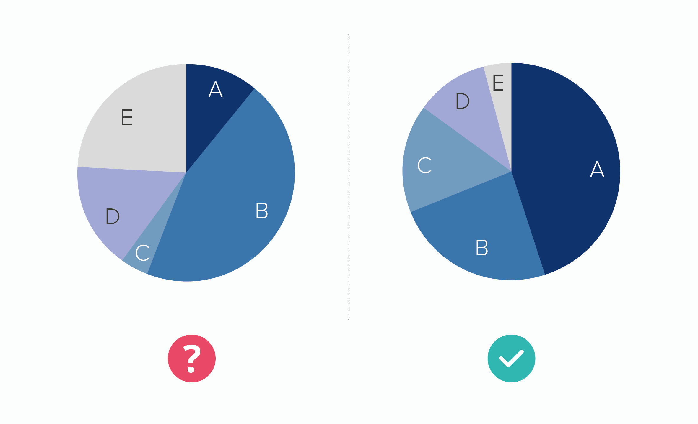
Rule 6 Arrange Your Pie Slices From Largest To Smallest Addtwo

Burn Rate Chart Earned Value Management Excel Templates

Work Time Management Pie Chart Effective Time Management Time Management Education Management

Rule 6 Arrange Your Pie Slices From Largest To Smallest Addtwo
How To Create Progress Charts Bar And Circle In Excel Automate Excel
1

Implementing Modular Spreadsheet Development A Walkthrough Spreadsheet Design Excel Dashboard Templates Dashboard Template

Rule 6 Arrange Your Pie Slices From Largest To Smallest Addtwo

Value Proposition Canvas Value Proposition Canvas Value Proposition Canvas